
An Efficient Soft-Margin Kernel SVM Implementation In Python
Published:
This short tutorial aims at introducing support vector machine (SVM) methods from its mathematical formulation along with an efficient implementation in a few lines of Python! Do play with the full code hosted on my github page. I strongly recommend reading Support Vector Machine Solvers (from L. Bottou & C-J. Lin) for an in-depth cover of the topic, along with the LIBSVM library. The present post naturally follows this introduction on SVMs.
Support Vector Machines - The model
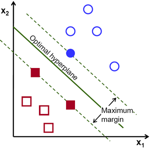
Figure 1: An optimal hyperplane.
As illustrated on Figure 1, SVMs represent examples as points in space, mapped so that the examples of the different categories are divided by a clear gap that is as wide as possible. New examples are then mapped into that same space and assigned a category based on which side of the gap they fall.
Let's consider a dataset $D = { (\mathbf{x}_{i}, y_{i}), \mathbf{x} \in \mathbb{R}^d, y \in \{ -1, 1 \}}$ , and $\phi$ a feature mapping - a possibly non-linear function used to get features from the datapoints $\{x_i\}$.
The main idea is to find an hyperplane $\w^*$ separating our dataset and maximising the margin of this hyperplane:
\begin{equation} \label{eq:hard_objective} \min _{\w, b} \mathcal{P}(\w, b) = \cfrac{1}{2} \w^2 \end{equation} \begin{equation} \label{eq:hard_conditions} \text{subject to} \ \forall i \ \ y_i(\w^T \phi(\x_i)+b) \ge 1 \end{equation} The conditions (\ref{eq:hard_conditions}) enforce that datapoints (after being mapped through $\phi$) from the first (respectively second) category lie below (respectively above) the hyperplane $\w^*$, while the objective (\ref{eq:hard_objective}) maximises the margin (the distance between the hyperplane $\w^*$ and the closest example).
Soft margin
We implicitly made the assumption that the dataset $D$ was separable: that there exists an hyperplane $\w^* \in \mathbb{R}^d$ such that all red points (i.e. $y=-1)$ lie on one side of the hyperplane (i.e. $\w^T \phi(\x_i)+b \le 0$) and blue points (y=$+1)$ lie on the other side of the hyperplane (i.e. $\w^T \phi(\x_i)+b \ge 0$).
This formulation is called hard margin, since the margin cannot let some datapoints go through (all datapoints are well classified).
This assumption can be relaxed by introducing positive slack variables $\mathbf{\xi}=(\xi_1, \dots, \xi_n)$
allowing some examples to violate the margin constraints (\ref{eq:hard_conditions}).
$\xi_i$ are non-zero only if $\x_i$ sits on the wrong side of the hyperplane, and is equal to the distance between $\x_i$ and the hyperplane $\w$.
Then an hyperparameter $C$ controls the compromise between large margins and small margin violations.
\begin{equation} \label{eq:hard_primal} \min _{\w, b, \mathbf{\xi}} \mathcal{P}(\w, b, \mathbf{\xi}) = \cfrac{1}{2} \w^2 + C \sum_{i=1}^n \xi_i \\ \text{subject to} \begin{cases} \forall i \quad y_i(\w^T \phi(\x_i)+b) \ge 1 - \xi_i \\ \forall i \quad \xi_i \ge 0 \end{cases} \end{equation}
How to fit the model ?
Once one have such a mathematical representation of the model through an optimisation problem, the next natural question arising is how should we solve this problem (once we know it is well-posed) ? The SVM solution is the optimum of a well defined convex optimisation problem (\ref{eq:hard_primal}). Since the optimum does not depend on the manner it has been calculated, the choice of a particular optimisation algorithm can be made on the sole basis of its computational requirements.
Dual formulation
Directly solving (\ref{eq:hard_primal}) is difficult because the constraints are quite complex. A classic move is then to simplify this problem via Lagrangian duality (see L. Bottou et al for more details), yielding the dual optimisation problem: \begin{equation} \label{eq:soft_dual} \max _{\alpha} \mathcal{D}(\alpha) = \sum_{i=1}^n \alpha_i - \cfrac{1}{2} \sum_{i,j=1}^n y_i \alpha_i y_j \alpha_j \mathbf{K}(\x_i, \x_j) \\ \end{equation} \begin{equation} \label{eq:soft_dual_cons} \text{subject to} \begin{cases} \forall i \quad 0 \le \alpha_i \le C \\ \sum_i y_i\alpha_i = 0 \end{cases} \end{equation} with $\{\alpha_i\}_{i=1,\dots,n}$ being the dual coefficients to solve and $\mathbf{K}$ being the kernel associated with $\phi$: $\forall i,j \ \ \mathbf{K}(\x_i, \x_j)=\left< \phi(\x_i) , \phi(\x_j)\right>$. That problem is much easier to solve since the constraints are much simpler. Then, the direction $\w^*$ of the optimal hyperplane is recovered from a solution $\alpha^*$ of the dual optimisation problem (\ref{eq:soft_dual}-\ref{eq:soft_dual_cons}) (by forming the Lagragian and taking its minimum w.r.t. $\w$ - which is a strongly convex function): \begin{equation} \w^* = \sum_{i} \alpha^*_i y_i \phi(\x_i) \end{equation} The optimal hyperplane is therefore a weighted combination over the datapoints with non-zero dual coefficient $\alpha^*_i$. Those datapoints are therefore called support vectors, hence «support vector machines». This property is quite elegant and really useful since in practice only a few $\alpha^*_i$ are non-zeros. Hence, a new datapoint prediction only requires to evaluate: \begin{equation} \text{sign}\left(\w^{*T} \phi(\x)+b\right) = \text{sign}\left(\sum_{i} \alpha^*_i y_i \phi(\x_i)^T\phi(\mathbf{x}) +b\right) = \text{sign}\left(\sum_{i} \alpha^*_i y_i \mathbf{K}(\mathbf{x}_i, \mathbf{x}) +b \right) \end{equation}
Quadratic Problem solver
The SVM optimisation problem (\ref{eq:soft_dual}) is a Quadratic Problem (QP), a well studied class of optimisation problems for which good libraries has been developed for.
This is the approach taken in this intro on SVM, relying on the Python's quadratic program solver cvxopt.
Yet this approach can be inefficient since such packages were often designed to take advantage of sparsity in the quadratic part of the objective function. Unfortunately, the SVM kernel matrix $\mathbf{K}$ is rarely sparse but sparsity occurs in the solution of the SVM problem.
Moreover, the specification of a SVM problem rarely fits in memory and generic optimisation packages sometimes make extra work to locate the optimum with high accuracy which is often useless.
Let's then described an algorithm tailored to efficiently solve that optimisation problem.
The Sequential Minimal Optimisation (SMO) algorithm
One way to avoid the inconveniences above-mentioned is to rely on the decomposition method.
The idea is to decompose the optimisation problem in a sequence of subproblems where only a subset of coefficients $\alpha_i$, $i \in \mathcal{B}$ needs to be optimised, while leaving the remaining coefficients $\alpha_j$, $j \notin \mathcal{B}$ unchanged:
\begin{equation} \label{eq:smo}
\max _{\alpha'} \mathcal{D}(\alpha') = \sum_{i=1}^n \alpha'_i - \cfrac{1}{2} \sum_{i,j=1}^n y_i \alpha'_i y_j \alpha'_j \mathbf{K}(\x_i, \x_j) \\
\text{subject to} \begin{cases} \forall i \notin \mathcal{B} \quad \alpha'_i=\alpha_i \\
\forall i \in \mathcal{B} \quad 0 \le \alpha'_i \le C \\
\sum_i y_i\alpha'_i = 0 \end{cases}
\end{equation}
One need to decide how to choose the working set $\mathcal{B}$ for each subproblem. The simplest is to always use the smallest possible working set, that is, two elements (such as the maximum violating pair scheme, which is discussed in Section 7.2 in Support Vector Machine Solvers ). The equality constraint $\sum_i y_i \alpha'_i = 0$ then makes this a one dimensional optimisation problem.
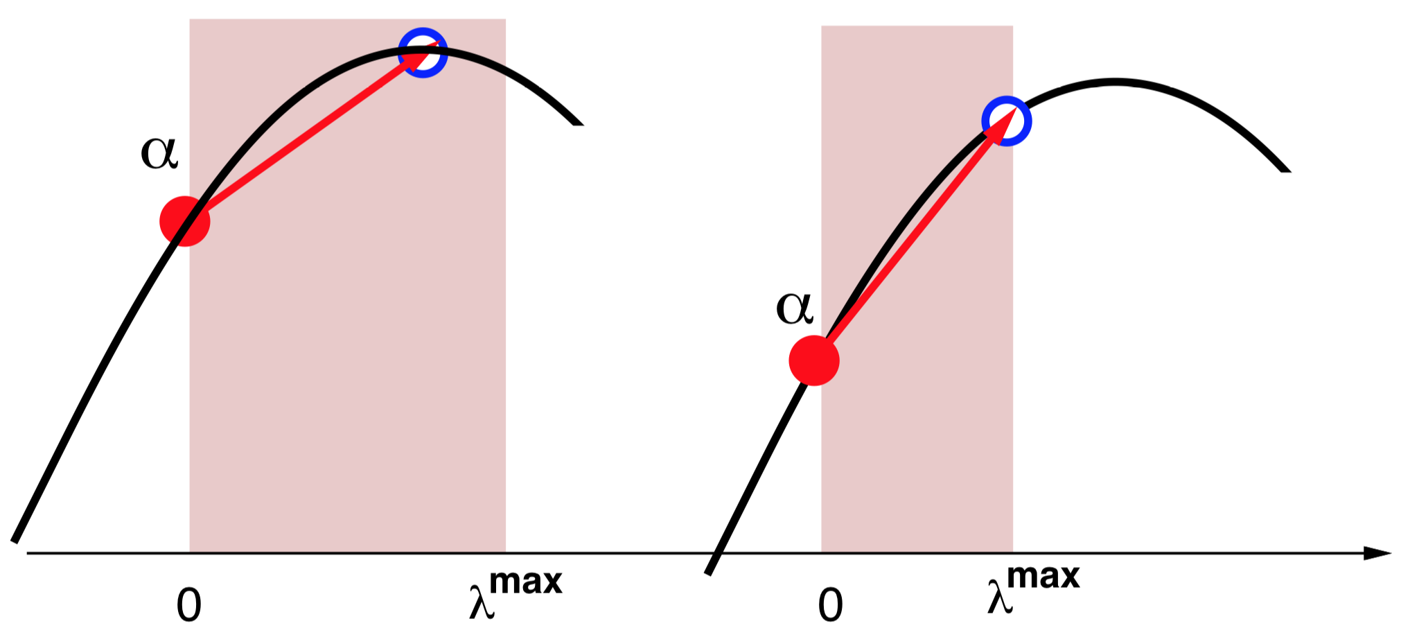
Figure 2: Direction search - from L. Bottou & C-J. Lin.
The equality constraint (\ref{eq:smo}) restricts $\mathbf{u}$ to the linear subspace $\sum_i y_i u_i = 0$. Each subproblem is therefore solved by performing a search along a direction $\mathbf{u}$ containing only two non zero coefficients: ${u}_i = y_i$ and ${u}_j = −y_j$.
The set $\Lambda$ of all coefficients $\lambda \ge 0$ is defined such that the point $\mathbf{\alpha} + \lambda \mathbf{u}$ satisfies the constraints. Since the feasible polytope is convex and bounded $\Lambda = [0, \lambda^{\max}]$. Direction search is expressed by the simple optimisation problem \begin{equation} \lambda^* = \arg\max_{\lambda \in \Lambda}{\mathcal{D}(\mathbf{\alpha }+ \lambda \mathbf{u})} \end{equation} Since the dual objective function is quadratic, $\mathcal{D}(\mathbf{\alpha }+ \lambda \mathbf{u})$ is shaped like a parabola. The location of its maximum $\lambda^+$ is easily computed using Newton’s formula: \begin{equation} \lambda^+ = \cfrac{ \partial \mathcal{D}(\mathbf{\alpha }+ \lambda \mathbf{u}) / \partial \lambda \ |_{\lambda=0} } {\partial^2 \mathcal{D}(\mathbf{\alpha }+ \lambda \mathbf{u}) / \partial \lambda^2 \ |_{\lambda=0}} = \cfrac{\mathbf{g}^T \mathbf{u}}{\mathbf{u}^T \mathbf{H} \mathbf{u}} \end{equation}
where vector $\mathbf{g}$ and matrix $\mathbf{H}$ are the gradient and the Hessian of the dual objective function $\mathcal{D}(\mathbf{\alpha})$: \begin{equation} g_i = 1 - y_i \sum_j{y_j \alpha_j K_{ij}} \quad \text{and} \quad H_{ij} = y_i y_j K_{ij} \end{equation} Hence $\lambda^* = \max \left(0, \min \left(\lambda^{\max}, \lambda^+ \right)\right) = \max \left(0, \min \left(\lambda^{\max}, \cfrac{\mathbf{g}^T \mathbf{u}}{\mathbf{u}^T \mathbf{H} \mathbf{u}} \right)\right)$.
Implementation
From a Python’s class point of view, an SVM model can be represented via the following attributes and methods:
Then the _compute_weights method is implemented using the SMO algorithm described above:
Demonstration
We demonstrate this algorithm on a synthetic dataset drawn from a two dimensional standard normal distribution. Running the example script will generate the synthetic dataset, then train a kernel SVM via the SMO algorithm and eventually plot the predicted categories.


Optimal hyperplane with predicted labels for radial basis (left) and linear (right) kernel SVMs.
The material and code is available on my github page. I hope you enjoyed that tutorial !
Acknowledgments
I’m grateful to Thomas Pesneau for his comments.